[1]:
import numpy as np
import os
import matplotlib.pyplot as plt
import matplotlib.ticker as ticker
from astropy.table import Table, join
from astropy import units as u
from edge_pydb import EdgeTable

params = {'mathtext.default': 'regular' }
plt.rcParams.update(params)
Plotting Global Properties
This notebook gives a few examples of plotting the CSV tables that are found in the dat_glob subdirectory of edge_pydb. These tables provided galaxy-wide properties from CALIFA or CARMA and are hence referred to as “global”.
Plot CO observation parameters, a la Bolatto et al. (2017) Figure 4.
[2]:
coobs = EdgeTable('edge_coobs_DE.csv')
coobs
[2]:
EdgeTable length=126
| Name | coVsys | coDEobstim | coNpt | coDEbmaj | coDEbmin | coRMS_10 | coTpk_10 | coSNRpeak_10 | ImagingDate_10 | coRMS_20 | coTpk_20 | coSNRpeak_20 | ImagingDate_20 |
|---|---|---|---|---|---|---|---|---|---|---|---|---|---|
| km / s | h | arcsec | arcsec | mK | mK | mK | mK | ||||||
| str13 | float64 | float64 | int64 | float64 | float64 | float64 | int64 | float64 | str21 | float64 | int64 | float64 | str21 |
| ARP220 | 5340.9 | 4.0 | 7 | 4.48 | 3.87 | 41.8 | 3472 | 83.03 | 02/14/16 05:15:10 CST | 33.0 | 3461 | 104.75 | 06/09/16 07:03:55 CDT |
| IC0480 | 4492.9 | 3.98 | 7 | 4.88 | 3.93 | 53.6 | 810 | 15.11 | 02/15/16 16:09:31 CST | 42.3 | 792 | 18.73 | 06/08/16 10:40:35 CDT |
| IC0540 | 2056.6 | 3.33 | 7 | 6.22 | 3.64 | 65.9 | 375 | 5.69 | 02/12/16 17:08:14 CST | 51.2 | 336 | 6.57 | 06/08/16 10:49:37 CDT |
| IC0944 | 6843.0 | 4.09 | 7 | 5.39 | 4.17 | 41.6 | 317 | 7.64 | 02/12/16 17:25:13 CST | 32.5 | 278 | 8.54 | 06/08/16 10:59:27 CDT |
| IC1151 | 2159.9 | 2.65 | 7 | 5.32 | 3.78 | 77.2 | 382 | 4.94 | 02/12/16 17:40:21 CST | 60.1 | 301 | 5.02 | 06/08/16 11:07:49 CDT |
| IC1199 | 4663.0 | 3.97 | 7 | 4.92 | 4.3 | 47.3 | 351 | 7.43 | 02/12/16 17:55:31 CST | 37.1 | 266 | 7.15 | 06/08/16 11:16:31 CDT |
| IC1683 | 4774.9 | 4.34 | 7 | 4.96 | 3.79 | 48.0 | 785 | 16.35 | 02/12/16 18:13:26 CST | 37.4 | 794 | 21.24 | 06/08/16 11:27:22 CDT |
| IC2247 | 4261.7 | 4.01 | 7 | 4.79 | 3.85 | 43.3 | 438 | 10.12 | 02/12/16 18:31:08 CST | 34.0 | 416 | 12.25 | 06/08/16 11:37:39 CDT |
| IC2487 | 4292.1 | 3.99 | 7 | 6.17 | 3.9 | 45.6 | 311 | 6.84 | 02/12/16 18:47:00 CST | 35.6 | 303 | 8.51 | 06/08/16 11:46:48 CDT |
| IC4566 | 5479.5 | 4.01 | 7 | 6.01 | 3.89 | 41.3 | 256 | 6.19 | 02/12/16 19:02:27 CST | 32.4 | 245 | 7.54 | 06/08/16 11:55:34 CDT |
| IC5376 | 4951.0 | 4.08 | 7 | 4.61 | 4.07 | 51.1 | 232 | 4.54 | 02/12/16 19:16:54 CST | 40.5 | 184 | 4.54 | 06/08/16 12:04:00 CDT |
| NGC0444 | 4762.1 | 3.14 | 7 | 5.03 | 4.1 | 57.5 | 265 | 4.61 | 02/12/16 19:32:20 CST | 45.7 | 202 | 4.43 | 06/08/16 12:12:45 CDT |
| NGC0447 | 5489.6 | 5.09 | 13 | 4.52 | 3.67 | 45.4 | 556 | 12.24 | 02/12/16 19:55:04 CST | 35.1 | 495 | 14.11 | 06/08/16 12:26:03 CDT |
| NGC0477 | 5751.4 | 4.33 | 7 | 5.11 | 3.93 | 50.5 | 325 | 6.44 | 02/12/16 20:17:28 CST | 39.5 | 273 | 6.9 | 06/08/16 12:38:12 CDT |
| NGC0496 | 5893.8 | 3.99 | 7 | 4.9 | 3.76 | 46.5 | 362 | 7.78 | 02/12/16 20:33:39 CST | 36.2 | 339 | 9.36 | 06/08/16 12:47:41 CDT |
| NGC0523 | 4683.0 | 4.3 | 7 | 4.63 | 3.77 | 58.5 | 640 | 10.93 | 02/12/16 20:50:59 CST | 43.8 | 572 | 13.08 | 06/08/16 12:57:29 CDT |
| NGC0528 | 4745.5 | 3.99 | 7 | 4.92 | 3.98 | 49.1 | 247 | 5.02 | 02/12/16 21:07:33 CST | 38.8 | 186 | 4.79 | 06/08/16 13:06:41 CDT |
| NGC0551 | 5113.3 | 3.94 | 7 | 4.8 | 3.79 | 46.1 | 329 | 7.12 | 02/12/16 21:23:38 CST | 35.7 | 282 | 7.89 | 06/08/16 13:15:46 CDT |
| NGC1167 | 4851.2 | 4.29 | 7 | 4.8 | 3.64 | 52.8 | 281 | 5.32 | 02/12/16 21:39:20 CST | 41.2 | 222 | 5.38 | 06/08/16 13:24:48 CDT |
| NGC2253 | 3542.0 | 3.99 | 7 | 5.65 | 4.15 | 45.8 | 671 | 14.65 | 02/12/16 21:57:48 CST | 36.1 | 619 | 17.16 | 06/08/16 13:35:06 CDT |
| NGC2347 | 4388.8 | 4.6 | 7 | 4.85 | 4.79 | 40.3 | 457 | 11.35 | 02/12/16 22:14:45 CST | 31.2 | 419 | 13.43 | 06/08/16 13:44:45 CDT |
| NGC2410 | 4602.2 | 7.35 | 13 | 4.92 | 4.06 | 54.5 | 344 | 6.3 | 02/12/16 22:37:42 CST | 42.9 | 299 | 6.97 | 06/08/16 13:58:11 CDT |
| NGC2480 | 2320.8 | 4.66 | 7 | 5.16 | 4.03 | 56.8 | 388 | 6.83 | 02/12/16 23:02:51 CST | 44.1 | 365 | 8.28 | 06/08/16 14:11:02 CDT |
| NGC2486 | 4569.7 | 1.3 | 7 | 4.6 | 3.89 | 88.6 | 451 | 5.09 | 02/12/16 23:19:01 CST | 69.6 | 329 | 4.72 | 06/08/16 14:19:23 CDT |
| NGC2487 | 4758.9 | 4.62 | 7 | 4.92 | 3.92 | 60.8 | 481 | 7.91 | 02/12/16 23:34:50 CST | 47.8 | 457 | 9.57 | 06/08/16 14:28:23 CDT |
| NGC2623 | 5437.6 | 6.23 | 14 | 5.18 | 3.84 | 30.6 | 1148 | 37.58 | 02/13/16 00:08:46 CST | 23.8 | 1109 | 46.5 | 06/08/16 14:47:52 CDT |
| NGC2639 | 3150.0 | 4.01 | 7 | 5.37 | 4.03 | 52.3 | 647 | 12.37 | 02/13/16 00:31:37 CST | 41.6 | 463 | 11.13 | 06/08/16 15:00:21 CDT |
| NGC2730 | 3795.1 | 4.31 | 7 | 5.55 | 4.06 | 48.4 | 271 | 5.61 | 02/13/16 00:46:25 CST | 37.4 | 211 | 5.63 | 06/08/16 15:08:43 CDT |
| ... | ... | ... | ... | ... | ... | ... | ... | ... | ... | ... | ... | ... | ... |
| UGC04280 | 3469.7 | 4.01 | 7 | 4.77 | 4.51 | 56.8 | 290 | 5.11 | 02/13/16 21:11:01 CST | 43.7 | 249 | 5.68 | 06/09/16 02:33:24 CDT |
| UGC04461 | 4906.5 | 3.99 | 7 | 4.88 | 4.22 | 53.1 | 376 | 7.09 | 02/13/16 21:27:23 CST | 41.4 | 352 | 8.52 | 06/09/16 02:42:51 CDT |
| UGC05108 | 7913.4 | 3.98 | 7 | 5.47 | 4.38 | 36.1 | 251 | 6.97 | 02/13/16 21:43:33 CST | 27.5 | 229 | 8.34 | 06/09/16 02:52:17 CDT |
| UGC05111 | 6595.5 | 4.61 | 7 | 5.21 | 4.95 | 37.6 | 403 | 10.7 | 02/13/16 22:00:36 CST | 29.4 | 373 | 12.7 | 06/09/16 03:01:45 CDT |
| UGC05244 | 2981.7 | 2.33 | 7 | 5.1 | 4.64 | 59.1 | 282 | 4.78 | 02/13/16 22:15:19 CST | 46.5 | 225 | 4.83 | 06/09/16 03:10:13 CDT |
| UGC05359 | 8249.5 | 3.99 | 7 | 6.75 | 4.87 | 27.8 | 150 | 5.42 | 02/13/16 22:29:51 CST | 21.6 | 125 | 5.76 | 06/09/16 03:18:33 CDT |
| UGC05498NED01 | 6174.4 | 3.93 | 7 | 5.24 | 3.92 | 61.9 | 273 | 4.41 | 02/13/16 22:44:36 CST | 47.8 | 250 | 5.23 | 06/09/16 03:26:43 CDT |
| UGC05598 | 5519.8 | 2.98 | 7 | 5.83 | 4.07 | 54.6 | 378 | 6.93 | 02/13/16 23:00:24 CST | 43.0 | 307 | 7.14 | 06/09/16 03:35:37 CDT |
| UGC06312 | 6201.5 | 2.94 | 7 | 4.61 | 4.57 | 50.8 | 224 | 4.4 | 02/13/16 23:15:55 CST | 39.5 | 189 | 4.78 | 06/09/16 03:43:53 CDT |
| UGC07012 | 3031.5 | 4.0 | 7 | 4.73 | 3.92 | 54.9 | 371 | 6.74 | 02/13/16 23:32:41 CST | 42.7 | 249 | 5.83 | 06/09/16 03:52:51 CDT |
| UGC08107 | 8076.9 | 3.88 | 7 | 4.87 | 4.47 | 36.3 | 304 | 8.37 | 02/25/16 17:47:43 CST | 28.2 | 272 | 9.67 | 06/09/16 04:02:41 CDT |
| UGC08250 | 5184.0 | 4.01 | 7 | 4.87 | 3.91 | 49.4 | 232 | 4.7 | 02/14/16 00:08:08 CST | 39.0 | 166 | 4.27 | 06/09/16 04:11:46 CDT |
| UGC08267 | 7078.6 | 4.27 | 7 | 4.7 | 3.92 | 50.9 | 471 | 9.26 | 02/14/16 00:25:41 CST | 39.7 | 445 | 11.2 | 06/09/16 04:21:29 CDT |
| UGC09067 | 7645.8 | 4.03 | 7 | 5.61 | 4.39 | 47.4 | 402 | 8.48 | 02/14/16 00:40:55 CST | 36.1 | 335 | 9.27 | 06/09/16 04:30:12 CDT |
| UGC09476 | 3236.1 | 4.0 | 7 | 5.16 | 3.89 | 58.1 | 313 | 5.39 | 02/14/16 00:56:11 CST | 45.2 | 243 | 5.39 | 06/09/16 04:38:44 CDT |
| UGC09537 | 8576.5 | 4.36 | 7 | 4.61 | 3.96 | 43.8 | 252 | 5.76 | 02/14/16 01:10:59 CST | 33.5 | 223 | 6.66 | 06/09/16 04:47:31 CDT |
| UGC09542 | 5386.6 | 3.98 | 7 | 5.06 | 3.61 | 53.1 | 313 | 5.89 | 02/14/16 01:26:49 CST | 41.0 | 289 | 7.04 | 06/09/16 04:56:27 CDT |
| UGC09665 | 2535.6 | 4.01 | 7 | 4.57 | 3.73 | 64.0 | 607 | 9.48 | 02/14/16 01:43:30 CST | 50.8 | 564 | 11.08 | 06/09/16 05:05:17 CDT |
| UGC09759 | 3408.4 | 3.97 | 7 | 5.04 | 3.67 | 54.0 | 655 | 12.13 | 02/14/16 02:00:47 CST | 42.1 | 620 | 14.73 | 06/09/16 05:14:47 CDT |
| UGC09873 | 5528.4 | 3.98 | 7 | 4.73 | 3.7 | 51.6 | 326 | 6.32 | 02/14/16 02:16:51 CST | 40.2 | 278 | 6.91 | 06/09/16 05:23:40 CDT |
| UGC09892 | 5569.7 | 3.67 | 7 | 4.84 | 4.15 | 44.8 | 215 | 4.81 | 02/14/16 02:32:45 CST | 34.5 | 194 | 5.6 | 06/09/16 05:32:06 CDT |
| UGC09919 | 3151.3 | 4.66 | 7 | 4.82 | 4.49 | 53.4 | 328 | 6.14 | 02/14/16 02:48:59 CST | 41.9 | 198 | 4.73 | 06/09/16 05:41:15 CDT |
| UGC10043 | 2153.2 | 4.29 | 7 | 4.67 | 3.9 | 69.3 | 614 | 8.85 | 02/14/16 03:05:49 CST | 54.1 | 610 | 11.26 | 06/09/16 05:50:59 CDT |
| UGC10123 | 3720.0 | 4.01 | 7 | 4.38 | 3.88 | 57.6 | 632 | 10.98 | 02/14/16 03:24:22 CST | 43.7 | 589 | 13.46 | 06/09/16 06:01:25 CDT |
| UGC10205 | 6432.9 | 2.96 | 7 | 5.57 | 4.14 | 44.5 | 232 | 5.22 | 02/14/16 03:39:42 CST | 34.4 | 213 | 6.17 | 06/09/16 06:09:41 CDT |
| UGC10331 | 4485.4 | 3.01 | 7 | 6.5 | 4.08 | 65.3 | 265 | 4.06 | 02/14/16 03:55:49 CST | 49.2 | 194 | 3.94 | 06/09/16 06:17:50 CDT |
| UGC10380 | 8510.7 | 4.01 | 7 | 4.82 | 4.38 | 46.5 | 237 | 5.1 | 02/14/16 04:10:49 CST | 35.9 | 226 | 6.28 | 06/09/16 06:26:18 CDT |
| UGC10384 | 4869.0 | 4.01 | 7 | 5.15 | 4.04 | 43.6 | 657 | 15.06 | 02/14/16 04:27:55 CST | 33.8 | 612 | 18.09 | 06/09/16 06:36:15 CDT |
| UGC10710 | 8153.9 | 4.01 | 7 | 5.04 | 3.95 | 50.5 | 367 | 7.28 | 02/14/16 04:42:31 CST | 38.4 | 236 | 6.16 | 06/09/16 06:44:41 CDT |
[3]:
plt.figure(figsize=(12, 7))

ax1=plt.subplot(2,3,1)
plt.hist(coobs['coDEobstim'], bins=np.arange(0, 20, 1), ec='black')
plt.xlabel('Observing time [h]', labelpad=2, fontsize='large')
plt.ylabel('Number of galaxies', labelpad=2, fontsize='large')
ax1.text(0.95,0.88,'$\mu$ = %3.1f h' % np.mean(coobs['coDEobstim']),
    ha='right',transform=ax1.transAxes)

ax2=plt.subplot(2,3,2)
beam=np.sqrt(coobs['coDEbmaj']*coobs['coDEbmin'])
plt.hist(beam, bins=np.arange(3, 6.2, 0.2), ec='black')
plt.xlabel('Beam size [arcsec]', labelpad=2, fontsize='large')
tick_spacing = 1
ax2.xaxis.set_major_locator(ticker.MultipleLocator(tick_spacing))
ax2.text(0.95,0.88,'$\mu$ = %3.1f"' % np.mean(beam),
    ha='right', transform=ax2.transAxes)

ax3=plt.subplot(2,3,3)
plt.hist(coobs['coRMS_10'], bins=np.arange(20,100,5), ec='black')
plt.xlabel('10 km/s Sensitivity [mK]', labelpad=2, fontsize='large')
ax3.text(0.95,0.88,'$\mu$ = %4.1f mK' % np.mean(coobs['coRMS_10']),
    ha='right', transform=ax3.transAxes)

ax4=plt.subplot(2,3,4)
plt.hist(coobs['coRMS_20'], bins=np.arange(20,100,5), ec='black')
plt.xlabel('20 km/s Sensitivity [mK]', labelpad=2, fontsize='large')
plt.ylabel('Number of galaxies', labelpad=2, fontsize='large')
ax4.text(0.95,0.88,'$\mu$ = %4.1f mK' % np.mean(coobs['coRMS_20']),
    ha='right', transform=ax4.transAxes)

ax5=plt.subplot(2,3,5)
plt.hist(coobs['coTpk_20'], bins=np.logspace(2,4,num=20), ec='black')
plt.xlabel('20 km/s Peak Signal [mK]', labelpad=2, fontsize='large')
ax5.set_xscale("log")
ax5.text(0.95,0.88,'$\mu$ = %4.1f mK' % np.mean(coobs['coTpk_20']),
    ha='right', transform=ax5.transAxes)

ax6=plt.subplot(2,3,6)
plt.hist(coobs['coSNRpeak_20'], bins=np.logspace(0.5,2,num=20), ec='black')
plt.xlabel('Peak SNR', labelpad=2, fontsize='large')
ax6.set_xscale("log")
ax6.text(0.95,0.88,'$\mu$ = %4.1f' % np.mean(coobs['coSNRpeak_20']),
    ha='right', transform=ax6.transAxes)

plt.subplots_adjust(hspace=0.25)
plt.show()

Derive \(S_{CO}\) to \(M_{mol}\) conversion.
[4]:
# Calculate molecular mass for 1 Jy km/s at 1 Mpc.
# These serve as fiducial distance and flux which we will scale later.
sco  = 1 * u.Jy * u.km / u.s
dmpc = (1 * u.Mpc).to(u.pc)
alphaco = 4.3 * u.solMass * u.s / (u.K * u.km * u.pc**2) # Bolatto+13
freq = 115.271204 * u.GHz
kperjy = (1*u.Jy/u.sr).to(u.K, equivalencies=u.brightness_temperature(freq))
molmass = alphaco * kperjy * (sco/u.Jy) * dmpc**2
print('At 1 Mpc, 1 Jy km/s of CO flux is {:.1f} of H_2'.format(molmass))
At 1 Mpc, 1 Jy km/s of CO flux is 10533.1 solMass of H_2
Plot derived CO masses, a la Bolatto et al. (2017) Figure 5. Need to merge in two additional tables.
[5]:
# Measured CO fluxes
natv_co = EdgeTable('edge_coflux_natv.csv')
# CALIFA params incl. distance
califa = EdgeTable('edge_califa.csv')
natv_co.join(califa)
natv_co.join(coobs)
WARNING: MergeConflictWarning: In merged column 'Name' the 'description' attribute does not match (Galaxy Name != CALIFA Name).  Using CALIFA Name for merged output [astropy.utils.metadata.merge]
WARNING: MergeConflictWarning: Cannot merge meta key 'date' types <class 'str'> and <class 'str'>, choosing date='2023-12-25' [astropy.utils.metadata.merge]
WARNING: MergeConflictWarning: Cannot merge meta key 'comments' types <class 'str'> and <class 'str'>, choosing comments='Galaxy properties determined from CALIFA' [astropy.utils.metadata.merge]
WARNING: MergeConflictWarning: In merged column 'Name' the 'description' attribute does not match (CALIFA Name != Galaxy Name).  Using Galaxy Name for merged output [astropy.utils.metadata.merge]
WARNING: MergeConflictWarning: Cannot merge meta key 'comments' types <class 'str'> and <class 'str'>, choosing comments='Observational Parameters for CARMA D+E array cubes' [astropy.utils.metadata.merge]
WARNING: MergeConflictWarning: Cannot merge meta key 'date' types <class 'str'> and <class 'str'>, choosing date='2023-06-20' [astropy.utils.metadata.merge]
[6]:
print(natv_co.colnames)
['Name', 'coRactr_natv', 'coDectr_natv', 'coCtrint_natv', 'coDvhel', 'coBmaj_natv', 'coBmin_natv', 'coBpa_natv', 'coNomask_natv', 'coeNomask_natv', 'coNomaskDv_natv', 'coDilated_natv', 'coeDilated_natv', 'coSmooth_natv', 'coeSmooth_natv', 'coSmoothDv_natv', 'coMask2d_natv', 'coeMask2d_natv', 'coSNRmax_natv', 'coSNR4pix_natv', 'coSNR5pix_natv', 'cottBmaj_natv', 'cottBmin_natv', 'cottBpa_natv', 'cottNomask_natv', 'cotteNomask_natv', 'cottNomaskDv_natv', 'cottDilated_natv', 'cotteDilated_natv', 'cottSmooth_natv', 'cotteSmooth_natv', 'cottSmoothDv_natv', 'cottMask2d_natv', 'cotteMask2d_natv', 'cottSNRmax_natv', 'cottSNR4pix_natv', 'cottSNR5pix_natv', 'ID', 'caSu', 'caSg', 'caSr', 'caSi', 'caB', 'caV', 'caR', 'caRe', 'caeRe', 'caEllipticity', 'caPA', 'caR50', 'caeR50', 'caR90', 'caeR90', 'cazgas', 'cazstars', 'caAge', 'caeAge', 'caFHa', 'caFHacorr', 'caLHacorr', 'caMstars', 'caeMstars', 'caSFR', 'caeSFR', 'caOH', 'caeOH', 'caAvgas', 'caeAvgas', 'caAvstars', 'caeAvstars', 'caDistP3d', 'caDistMpc', 'caFlgWav5', 'caFlgWav12', 'caFlgReg5', 'caFlgReg12', 'caFlgImg5', 'caFlgImg12', 'coVsys', 'coDEobstim', 'coNpt', 'coDEbmaj', 'coDEbmin', 'coRMS_10', 'coTpk_10', 'coSNRpeak_10', 'ImagingDate_10', 'coRMS_20', 'coTpk_20', 'coSNRpeak_20', 'ImagingDate_20']
[7]:
fig=plt.figure(figsize=(15, 4))

# Histogram of distance
ax1=plt.subplot(1,4,1)
plt.hist(natv_co['caDistMpc'],bins=np.arange(10, 150, 10), ec='black')
plt.xlabel('Distance [Mpc]', labelpad=3, fontsize='large')
plt.ylabel('Number of galaxies', labelpad=3, fontsize='large')
tick_spacing = 2
ax1.yaxis.set_major_locator(ticker.MultipleLocator(tick_spacing))
ax1.text(0.95,0.88,'$\mu$ = %3.1f' % np.mean(natv_co['caDistMpc']),
    ha='right', transform=ax1.transAxes)

# Histogram of beam physical size
ax2=plt.subplot(1,4,2)
beam = (np.sqrt(natv_co['coBmaj_natv']*natv_co['coBmin_natv'])).to(u.rad)
bmkpc = beam.value*natv_co['caDistMpc']*1000.
plt.hist(bmkpc,bins=np.arange(0, 4, 0.25), ec='black')
plt.xlabel('beam [kpc]', labelpad=3, fontsize='large')
ax2.text(0.95,0.88,'$\mu$ = %3.1f' % np.mean(bmkpc),
    ha='right', transform=ax2.transAxes)

# Histogram of beam mass sensitivity
ax3=plt.subplot(1,4,3)
# Convert mK to Jy/bm
omega_B = np.pi/(4*np.log(2)) * beam**2
conv = (u.Jy/omega_B).to(u.mK, equivalencies=u.brightness_temperature(freq))
mkperjy = conv.value
# Multiply 10 km/s noise by sqrt(3) to get sensitivity to a 30 km/s line
# Multiply by 4 to get 4-sigma sensitivity
msens = 4*molmass*(natv_co['caDistMpc']**2)*(natv_co['coRMS_10']/mkperjy)*10.*np.sqrt(3)
plt.hist(msens.value,bins=np.logspace(6, 9, num=20), ec='black')
plt.xlabel('$M_{sen,beam}$ [$M_\odot$]', labelpad=3, fontsize='large')
ax3.set_xscale("log")
ax3.text(0.95,0.88,'$\mu$ = %4.1e' % np.mean(msens.value),
    ha='right', transform=ax3.transAxes)

# Histogram of molecular gas mass
ax4=plt.subplot(1,4,4)
mgas = molmass*natv_co['caDistMpc']**2*natv_co['coSmooth_natv']
mgas = mgas[~np.isnan(mgas)]
plt.hist(mgas.value,bins=np.logspace(7.5, 11.5, num=20), ec='black')
plt.xlabel('$M_{mol}$ [$M_\odot$]', labelpad=3, fontsize='large')
ax4.set_xscale("log")
ax4.yaxis.set_major_locator(ticker.MultipleLocator(tick_spacing))
ax4.text(0.95,0.88,'$\mu$ = %4.1e' % np.mean(mgas.value),
    ha='right', transform=ax4.transAxes)

plt.show()

CO fluxes from 7” resolution cubes
[8]:
db = EdgeTable('edge_coflux_smo7.csv')
db.join(califa)
print('Stellar mass units:', db['caMstars'].unit)
print('SFR units:', db['caSFR'].unit)
Stellar mass units: dex(solMass)
SFR units: dex(solMass / yr)
[9]:
# Define the subsets
valid_ssfr = (~np.isnan(db['caMstars'])) & (~np.isnan(db['caSFR']))
valid_mgas = (~np.isnan(db['caMstars'])) & (~np.isnan(db['caSFR']))
co_det  = valid_ssfr & (~np.isnan(db['coDilated_smo7']))
print('Number of CO detections:',np.count_nonzero(co_det))
co_ndet = valid_ssfr & (np.isnan(db['coDilated_smo7']))
print('Number of CO non-detections:',np.count_nonzero(co_ndet))
Number of CO detections: 105
Number of CO non-detections: 21
[10]:
# Scale noise estimate from unmasked moment map to a more realistic velocity window
print('Median unmasked velocity width is',np.nanmedian(db['coNomaskDv_smo7']))
print('Median masked velocity width is',np.nanmedian(db['coDilatedDv_smo7']))
nsefactor = np.sqrt(np.nanmedian(db['coDilatedDv_smo7'])/np.nanmedian(db['coNomaskDv_smo7']))
print('Noise estimates will be scaled down by',nsefactor)
Median unmasked velocity width is 860.0
Median masked velocity width is 400.0
Noise estimates will be scaled down by 0.6819943394704735
[11]:
# Calculate gas mass, gas fraction, and offset from SFMS
# Main sequence from Cano-Diaz et al. (2016ApJ...821L..26C)
delsfr  = db['caSFR'] - (0.81*db['caMstars']-8.34)
mgas = np.log10(molmass.value * db['coDilated_smo7'] * db['caDistMpc']**2)
mgas[co_ndet] = np.log10(molmass.value *
                         2*nsefactor*db['coeNomask_smo7'][co_ndet]
                         * db['caDistMpc'][co_ndet]**2)
fgas = mgas - db['caMstars']
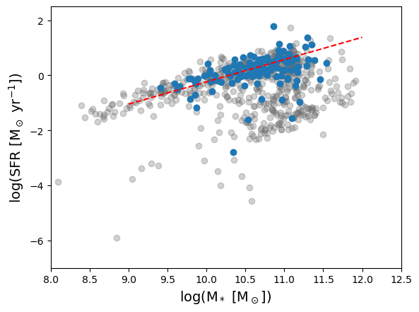
Scatterplots related to star-forming main sequence
[12]:
plt.scatter(califa['caMstars'],califa['caSFR'], c='dimgrey', alpha=0.3)
plt.scatter(db['caMstars'][valid_ssfr],db['caSFR'][valid_ssfr], c='tab:blue')
x_ms = np.linspace(9,12,num=50)
# Main sequence from Cano-Diaz et al. (2016ApJ...821L..26C)
y_ms = 0.81*x_ms-8.34
plt.plot(x_ms,y_ms,'r--')
plt.xlabel('log($M_*$ [$M_\odot$])', fontsize=14)
plt.ylabel('log(SFR [$M_\odot$ yr$^{-1}$])', fontsize=14)
plt.xlim(8,12.5)
plt.ylim(-7,2.5)
[12]:
(-7.0, 2.5)
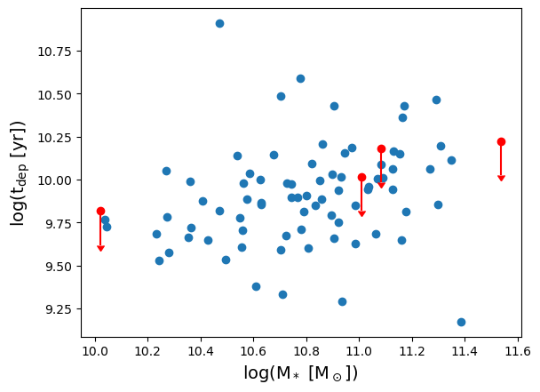
[13]:
tgaslg = mgas.value - np.log10(db['caSFR'].value)
plt.scatter(db['caMstars'][co_det], tgaslg[co_det])
plt.scatter(db['caMstars'][co_ndet],tgaslg[co_ndet],color='red')
uplims = np.ones(db['caMstars'][co_ndet].shape)
plt.errorbar(db['caMstars'][co_ndet],tgaslg[co_ndet], uplims=uplims,
             yerr=0.2, ls='none', color='red')
plt.xlabel('log($M_*$ [$M_\odot$])', fontsize=14)
plt.ylabel('log($t_{dep}$ [yr])', fontsize=14)
/var/folders/dr/623sc0b554s_rzxllbc_9tqc0000gn/T/ipykernel_8519/1255045184.py:1: RuntimeWarning: invalid value encountered in log10
  tgaslg = mgas.value - np.log10(db['caSFR'].value)
[13]:
Text(0, 0.5, 'log($t_{dep}$ [yr])')
[14]:
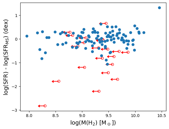
plt.scatter(mgas[co_det], delsfr[co_det])
plt.scatter(mgas[co_ndet],delsfr[co_ndet], facecolors='none',
            edgecolors='r', zorder=-1)
uplims = np.ones(mgas[co_ndet].shape)
plt.errorbar(mgas[co_ndet],delsfr[co_ndet], xuplims=uplims,
             xerr=0.1, ls='none', color='red', zorder=-2)
plt.ylabel(r'log(SFR) - log(SFR$_{\rm MS}$) (dex)', fontsize=14)
plt.xlabel('log($M(H_2)$ [$M_\odot$])', fontsize=14)
[14]:
Text(0.5, 0, 'log($M(H_2)$ [$M_\\odot$])')
[15]:
plt.scatter(fgas[co_det], delsfr[co_det])
plt.scatter(fgas[co_ndet],delsfr[co_ndet], facecolors='none',
            edgecolors='r', zorder=-1)
uplims = np.ones(fgas[co_ndet].shape)
plt.errorbar(fgas[co_ndet],delsfr[co_ndet], xuplims=uplims,
             xerr=0.1, ls='none', color='red', zorder=-2)
plt.ylabel(r'log(SFR) - log(SFR$_{\rm MS}$) (dex)', fontsize=14)
plt.xlabel('log($M(H_2)/M_*$)', fontsize=14)
[15]:
Text(0.5, 0, 'log($M(H_2)/M_*$)')

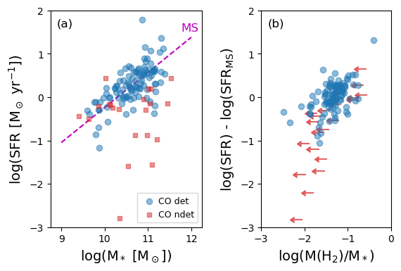
Database paper plot, EDGE only
[16]:
fig, (ax1,ax2) = plt.subplots(1,2, figsize=(7,4))

# Plot the data
ax1.scatter(db['caMstars'][co_det],db['caSFR'][co_det],
            c='tab:blue', alpha=0.5, label='CO det')
ax1.scatter(db['caMstars'][co_ndet],db['caSFR'][co_ndet], marker='s',
            c='tab:red', alpha=0.5, s=20, label='CO ndet')

# Main sequence from Cano-Diaz et al. (2016ApJ...821L..26C)
x_ms = np.linspace(9,12,num=50)
y_ms = 0.81*x_ms-8.34
ax1.plot(x_ms,y_ms,'m--', zorder=-2)
ax1.legend(loc='lower right', handletextpad=0.01, fontsize=9)

# Axis labels
ax1.set_xlabel('log($M_*$ [$M_\odot$])', fontsize=14)
ax1.set_ylabel('log(SFR [$M_\odot$ yr$^{-1}$])', fontsize=14)
ax1.set_aspect('equal')
ax1.set_xlim(8.75,12.25)
ax1.set_ylim(-3,2)

# Annotations
ax1.text(0.04,0.94, '(a)', size=12, ha='left',
         va='center', transform=ax1.transAxes)
ax1.text(0.92,0.92, 'MS', size=12, ha='center', color='m',
         va='center', transform=ax1.transAxes)

# Plot the data
ax2.scatter(fgas[co_det],delsfr[co_det],c='tab:blue', alpha=0.5)

# Plot the upper limits
uplims = np.ones(fgas[co_ndet].shape)
ax2.errorbar(fgas[co_ndet], delsfr[co_ndet], xuplims=uplims,
             xerr=0.2, ls='none', color='tab:red', zorder=-2, alpha=0.7)

# Axis labels
ax2.set_ylabel(r'log(SFR) - log(SFR$_{\rm MS}$)', fontsize=14)
ax2.set_xlabel('log($M(H_2)/M_*$)', fontsize=14)
ax2.set_aspect('equal')
ax2.set_xlim(-3,0)
ax2.set_ylim(-3,2)
ax2.text(0.05,0.94, '(b)', size=12, ha='left', va='center', transform=ax2.transAxes)

plt.subplots_adjust(wspace=0.1)
plt.savefig('sfms.pdf', bbox_inches='tight')
Database paper plot, EDGE+DR3
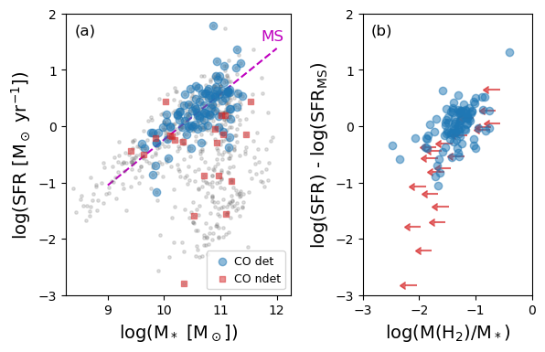
[17]:
fig, (ax1,ax2) = plt.subplots(1,2, figsize=(7.25,4))

# Plot the data
ax1.scatter(califa['caMstars'],califa['caSFR'], c='dimgrey', s=6, alpha=0.2)
ax1.scatter(db['caMstars'][co_det],db['caSFR'][co_det],
            c='tab:blue', alpha=0.5, label='CO det')
ax1.scatter(db['caMstars'][co_ndet],db['caSFR'][co_ndet], marker='s',
            c='tab:red', alpha=0.5, s=20, label='CO ndet')

# Main sequence from Cano-Diaz et al. (2016ApJ...821L..26C)
x_ms = np.linspace(9,12,num=50)
y_ms = 0.81*x_ms-8.34
ax1.plot(x_ms,y_ms,'m--', zorder=-2)
ax1.legend(loc='lower right', handletextpad=0.01, fontsize=9)

# Axis labels
ax1.set_xlabel('log($M_*$ [$M_\odot$])', fontsize=14)
ax1.set_ylabel('log(SFR [$M_\odot$ yr$^{-1}$])', fontsize=14)
ax1.set_aspect('equal')
ax1.set_xlim(8.25,12.25)
ax1.set_ylim(-3,2)

# Annotations
ax1.text(0.04,0.94, '(a)', size=12, ha='left',
         va='center', transform=ax1.transAxes)
ax1.text(0.92,0.92, 'MS', size=12, ha='center', color='m',
         va='center', transform=ax1.transAxes)

# Plot the data
ax2.scatter(fgas[co_det],delsfr[co_det],c='tab:blue', alpha=0.5)

# Plot the upper limits
uplims = np.ones(fgas[co_ndet].shape)
ax2.errorbar(fgas[co_ndet], delsfr[co_ndet], xuplims=uplims,
             xerr=0.2, ls='none', color='tab:red', zorder=-2, alpha=0.7)

# Axis labels
ax2.set_ylabel(r'log(SFR) - log(SFR$_{\rm MS}$)', fontsize=14)
ax2.set_xlabel('log($M(H_2)/M_*$)', fontsize=14)
ax2.set_aspect('equal')
ax2.set_xlim(-3,0)
ax2.set_ylim(-3,2)
ax2.text(0.05,0.94, '(b)', size=12, ha='left', va='center', transform=ax2.transAxes)

plt.subplots_adjust(wspace=0.1)
plt.savefig('sfms_dr3.pdf', bbox_inches='tight')
[ ]: